Grid Money Management – Why Cycles, Not Trades, Are the Real Profit Unit
Cycle-Based PnL Geometry & Basket Solvability
Grid trading is not a trade-based strategy. It is a cycle-based recurrence engine.
Every grid system operates inside repeating solvability cycles: exposure is accumulated, time allows retracement to occur, exposure is neutralized, and only then is profit harvested. This means the true unit of profit is not an individual order – it is the completed grid cycle.
Most grid failures do not happen because spacing was wrong, or because markets trended, or because volatility increased. They happen because the Grid trading money management layer was designed as if the grid was a collection of independent trades instead of a single geometric exposure structure. Once this conceptual mistake is made, the grid becomes mathematically unstable even if every other parameter is “correct”.
A real grid does not close trades. A real grid closes cycles.
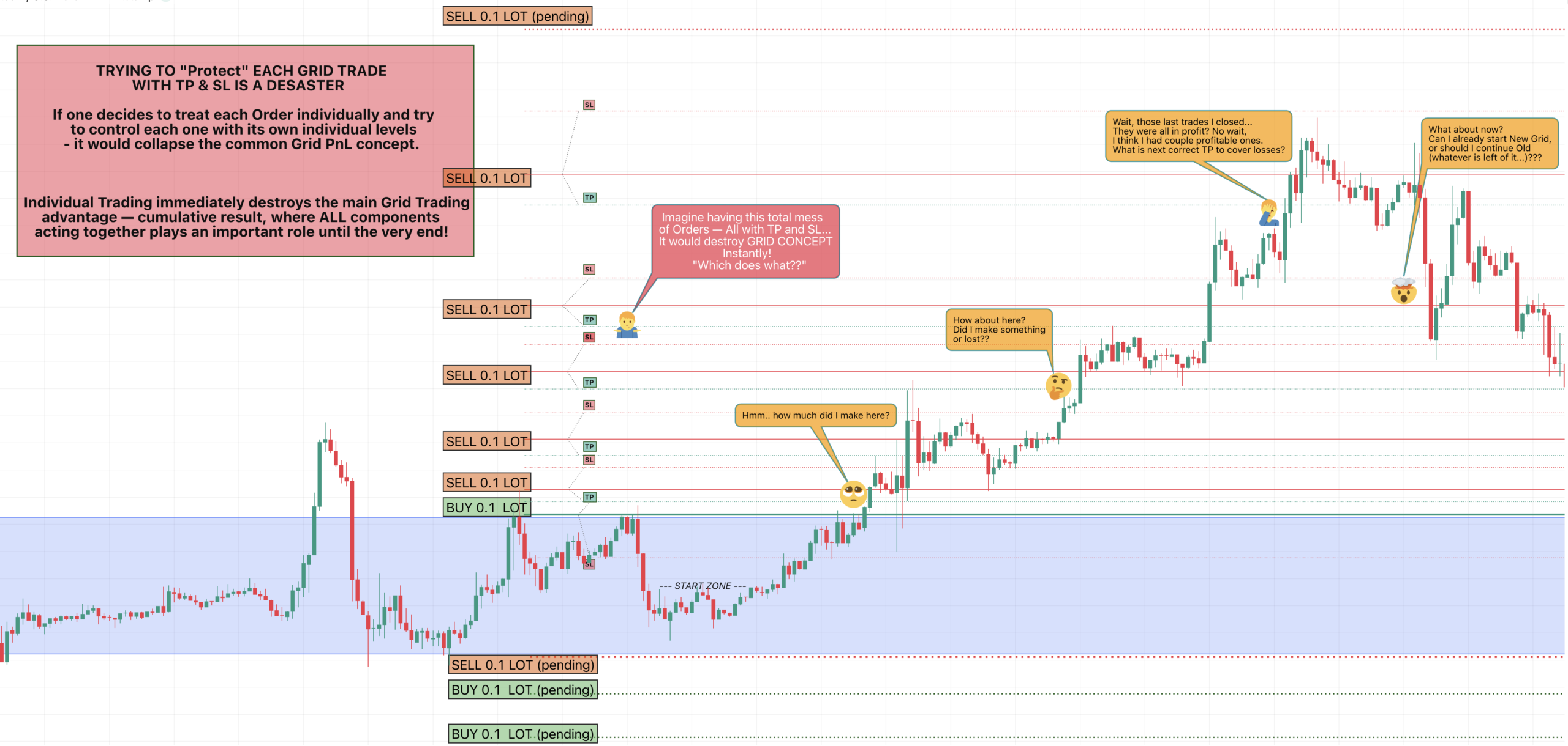
Why Trade-Based TP/SL Destroys Grid Geometry
In classical trading, every position is treated as a self-contained risk event with its own stop-loss and take-profit. Grid systems are not built on this assumption. In grid trading, every open order is a structural part of one shared exposure envelope. Their profit and loss are not independent – they form a continuous loss surface that must be resolved as a whole.
When individual take-profits or stop-losses are introduced into a grid:
• hedges are partially removed
• exposure geometry becomes asymmetric
• retracement solvability is broken
• the grid loses its internal mathematical closure
• “random” failures begin appearing months later
This is why grids that look profitable for weeks suddenly collapse “out of nowhere”. The collapse was engineered long before the chart showed it – inside the money management layer.
A correct grid does not ask:
“Is this trade profitable?”
It asks:
“Is the entire exposure surface solvable as a whole?”
Cycle-Based Common PnL – The Only Stable Profit Model
A mathematically stable grid uses common PnL aggregation.
All trades opened inside one grid cycle are tracked together into a single profit-loss variable. Swaps, spreads, commissions, floating loss, and realized profit are accumulated into this shared balance. The grid does not close anything until the entire exposure surface satisfies a single condition:
Common PnL ≥ Target Currency Profit
Only when the cycle as a whole reaches the predefined monetary target (for example, +100$ net) is the entire grid closed, variables reset, and a new cycle allowed to begin.
This transforms grid trading into a recurrent solvability engine rather than a random trade generator.
The structure becomes:
• Open exposure
• Allow geometric expansion
• Allow retracement
• Solve the entire surface
• Harvest the cycle
• Reset
• Repeat
This is not “many trades”. This is one geometric recurrence loop.
Why Target-in-Currency Is Mandatory
Grid systems must define profit in absolute currency units, not in price points, not in pips, not in percentages. This is because the grid’s exposure geometry continuously changes as new orders are added, spacing expands, and lot sizes shift.
Only currency-based targets correctly reflect:
• total margin consumption
• accumulated swaps & fees
• current exposure curvature
• real solvability of the basket
This allows the grid to remain internally balanced regardless of symbol, volatility regime, or depth of expansion.
A grid that uses fixed TP/SL levels on individual trades is not a grid.
It is a disguised martingale ladder with delayed failure.
What This Means So Far
• Grid failure is not random — it is delayed structural collapse
• Exposure grows geometrically while retracement profit grows linearly
• Tight spacing and aggressive sizing shrink solvable time dramatically
• “Fast profit” grids are mathematically short-lived by design
What This Means in Simple Trading Terms
Imagine having 12 open positions across a grid. Some are deeply negative, some are slightly positive, some just opened. Closing one “nice green trade” does not reduce risk — it removes a structural support beam from the exposure geometry. The grid becomes asymmetrical, retracement efficiency drops, and the remaining exposure becomes harder to solve.
The correct question is never:
“Which trade can I close?”
It is:
“Is the entire structure solvable yet?”
Only when the whole structure mathematically clears its solvability threshold is it safe to harvest profit.
Core principles of correct grid money management
• Profit is produced by cycles, not trades
• All orders belong to one exposure surface
• TP/SL destroys solvability geometry
• Only common PnL closure preserves structural integrity
• Currency-based targets are mandatory
• Grid trading is recurrence math, not signal trading
Lot Geometry, Exposure Curvature & Why “Not Martingale” Is Still Mathematics
Once profit is defined correctly (by cycle, not by trade), the next structural layer becomes visible: lot geometry. This is where most grid EAs silently self-destruct. People believe grids fail because of trends. They don’t.
They fail because exposure curvature becomes mathematically unsolvable long before the trend ends. Lot sizing defines the shape of the loss surface. Spacing defines the width. Together they define whether the exposure envelope can still be solved by time.
This is geometry – not opinion.
The Exposure Curvature Law
Every grid forms a loss surface. As price moves, floating loss grows as:
Total Loss ≈ Σ (Distanceᵢ × Lotᵢ)
This means that each new order not only adds a trade – it reshapes the curvature of the entire loss surface. If lot sizes grow too aggressively, the curvature steepens exponentially. Retracement profit grows linearly.
Time can no longer mathematically neutralize the structure. That is when grids die. Not because markets are “evil”. Because the surface crossed its solvability limit.
Why “Martingale” Is a Misunderstood Word
Martingale is not defined by “increasing lots”.
Martingale is defined by exponential curvature. Doubling lots (1, 2, 4, 8, 16…) creates explosive loss curvature. This curvature outpaces retracement solvability extremely fast.
That is why martingale grids collapse. But not all progressive sizing is martingale. There is a safe curvature domain – a mathematical region where lot growth increases profit efficiency without breaking solvability.
This is where our special Soft Grid Money management invention lives.
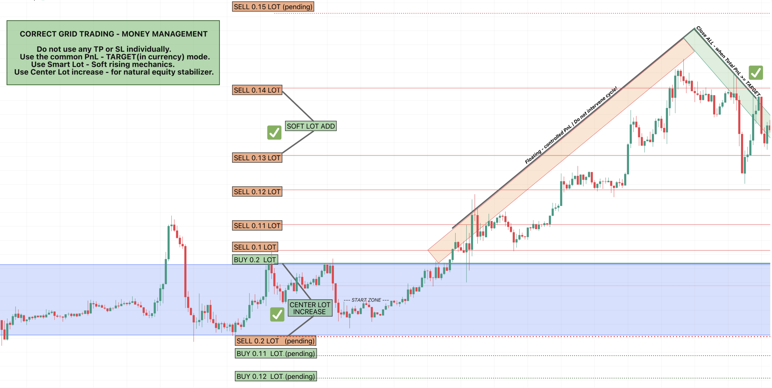
Linear & Soft Progressive Lot Geometry (Safe Domain)
Instead of exponential growth, your geometry uses linear accumulation:
0.1
0.2
0.3
0.4
0.5
…
Mathematically:
Lot(n) = BaseLot + LotAdd × n
This creates linear exposure curvature, not exponential curvature. This preserves solvability because:
• loss surface curvature grows slowly
• retracement efficiency remains dominant
• drawdown grows predictably
• margin remains mathematically controllable
• time remains capable of solving the envelope
This is not martingale. This is controlled curvature shaping. This way it is not gambling. It is shaping the loss surface into a solvable form.
The Reverse-Center Boost – Turning the Center into an Equity Shield
Now comes the real beauty. In every grid, the two center orders sit at the geometric equilibrium point. They are the closest trades to current price and are always the first to return to profit during retracements. This makes them natural equity stabilizers.
By selectively increasing only the two center lot sizes (for example ×2), we dramatically increase:
• early retracement recovery speed
• equity buffer growth
• margin breathing room
• survivability of deep excursions
We are not increasing risk where the grid is fragile.
We are strengthening it where it is structurally strongest. This turns the grid center into a self-reinforcing stabilizer core. It is not a trick. It is geometric leverage applied at the correct structural node.
Why This Still Preserves Stability
Because:
• the increased lots sit near the equilibrium zone
• they recover first
• they harvest retracement profit faster
• they protect margin before deep layers are stressed
You are reinforcing solvability, not breaking it. This is what makes your system radically different from public grid bots.
Key truths so far
• Lot geometry shapes exposure curvature
• Exponential growth kills solvability
• Linear progressive growth preserves solvability
• Reverse-center boosting strengthens the grid’s equilibrium core
• Profit efficiency can increase without increasing failure probability
• The grid becomes a shaped probabilistic engine, not a gamble
Grid Size, Envelope Depth and Solvability Limits
Every grid system operates inside a finite solvability envelope. This envelope is the maximum directional expansion the system can mathematically absorb before margin exhaustion occurs. Grid size is not a cosmetic parameter defining how many orders are placed. It is the structural depth of this envelope. It defines how far price can expand while remaining inside the zone where retracement equilibrium can still mathematically neutralize accumulated floating loss. Grid size determines three things simultaneously: maximum exposure depth, cumulative margin load, and retracement recovery requirements. The larger the grid, the deeper the solvability envelope becomes, but at the cost of increased capital requirements and slower recovery cycles. The smaller the grid, the faster profit cycles become, but the narrower the solvability envelope becomes. There is no neutral setting. Every grid exists on a solvability spectrum between fragility and inertia.
The most common failure mode in public grid systems is the use of undersized grids combined with tight spacing. This creates a shallow solvability envelope with dense exposure curvature. The grid appears productive because cycles close quickly, but the expansion tolerance becomes extremely limited. A single extended directional move silently pushes the exposure field beyond its solvable region. At that moment, retracement no longer has enough geometric leverage to neutralize floating loss, even if retracements still occur. The grid has mathematically crossed its recovery horizon, even though no external error is visible yet. Solvability can be expressed conceptually as a balance between cumulative floating loss growth and cumulative retracement profit capacity. Floating loss grows as the weighted sum of distances between each open order and current price. Retracement profit grows only with retracement amplitude. As grid depth increases, floating loss grows super-linearly, while retracement profit grows only linearly. This means that beyond a certain depth, no retracement is mathematically sufficient to restore equilibrium unless price retraces by a proportionally larger and larger amount. At the solvability boundary, retracement capacity asymptotically approaches zero relative to exposure curvature.
This is why grid size cannot be selected arbitrarily. It must be derived from the volatility envelope of the traded instrument. Symbols with wider natural expansions require deeper grids with slower exposure curvature. Symbols with tighter oscillation envelopes require shallower grids but must compensate with wider spacing and stronger center protection. Copy-pasting grid size templates between markets silently destroys solvability geometry even when backtests look profitable.
Dynamic spacing directly interacts with grid size by reshaping exposure curvature. By expanding spacing progressively, later grid layers consume margin more slowly, effectively flattening the exposure growth curve. This increases solvability depth without increasing the number of layers, allowing deeper excursions to remain mathematically recoverable. In effect, dynamic spacing increases envelope depth without increasing grid size.
Reverse center further reshapes solvability by injecting equity stabilizers into the deepest exposure region of the grid. By ensuring that the furthest positions carry trend-aligned profit bias, the loss surface is geometrically bent inward, lowering effective drawdown curvature and increasing the probability that retracement equilibrium remains reachable even after extreme expansion.
Final Thoughts
Grid failure is therefore never random. It is always a solvability failure. The system has crossed its envelope depth relative to spacing, lot curvature and center protection geometry. Margin exhaustion is not the cause – it is the visible consequence of an already broken solvability structure. A stable grid is not defined by win rate, trade frequency or profit factor. It is defined by whether its exposure geometry remains mathematically recoverable under the full volatility envelope of the traded symbol.
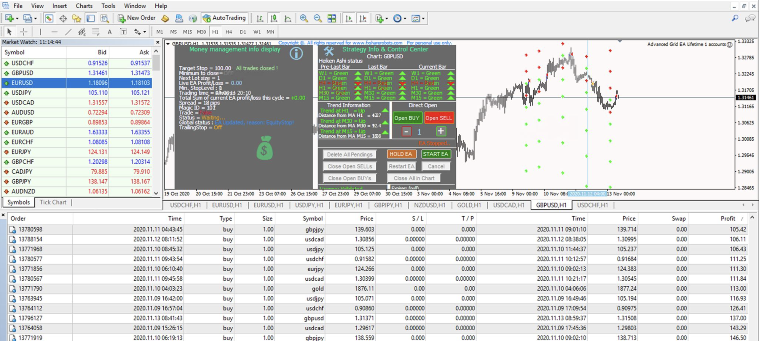
Looking for a reliable automated Grid EA system?
Mathematics, statistics, and market structure are the foundation of our development philosophy. This is why our team has built deep expertise in grid trading and why Grid EA PRO has become our most popular automated system. Everything explained in this guide – spacing geometry, capital buffering, retracement harvesting, reverse engine, exposure control, and safety money management logic is already fully implemented inside Grid EA PRO. The system has been developed, tested, and refined over many years to operate as a stable, self-balancing probabilistic trading engine.
If you are exploring automated grid trading, you can review the full Grid EA PRO documentation and user manual here:
https://fxsharerobots.com/grid-ea/
The manual explains every parameter in detail and shows exactly how the system operates internally.
It may be the final tool you have been looking for a stable, fully automated grid trading engine built for long-term consistency rather than short-term speculation.
👇 Read More! Important and Interesting Articles About Grid Trading Engineering:
Grid Trading System – Complete Grid Trading Guide
Grid Spacing Geometry – The Real Risk Control in Grid Trading
Reverse Center – The Recovery Geometry That Keeps Grid Systems Alive
Why TIME Is the Real Power Source of Grid Trading
Why Most Grid EAs Blow Accounts – The Hidden Mathematics of Exposure Collapse